Paper & Results¶

SoRoMoX is presented in “SoRoMoX: Fast, Differentiable, and Parallelizable Soft Robot Models”.

Using SoRoMoX in research?

The Citation guide provides the recommended paper BibTeX, an exact-version software citation, and model- or controller-specific references.

Paper overview¶

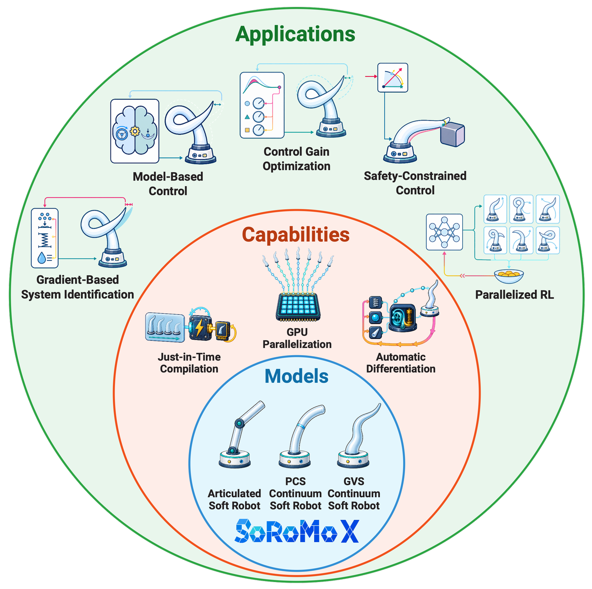
The paper's primary contribution is a fully numerical, JIT-compilable Python/JAX implementation of control-oriented models for articulated and continuum soft robots. SoRoMoX implements articulated soft-robot, piecewise-constant strain (PCS), and geometric variable strain (GVS) models through one interface for kinematics, dynamics, energies, Jacobians and derivatives, actuation maps, and forward dynamics.

Because the numerical core is JAX-native, these model computations can be JIT-compiled, automatically differentiated with respect to states, inputs, and physical parameters, vectorized, and executed on CPUs, GPUs, and TPUs. Model-based controllers and rendering backends are supporting contributions built around this model layer.

Overview of SoRoMoX model families, JAX-native numerical infrastructure, and application case studies — SoRoMoX brings control-oriented articulated, PCS, and GVS models into the JAX computational stack.

Model evaluation¶

Sequential CPU rollouts¶

The paper reports wall-clock time for three seconds of simulated motion. The table below retains the matched PCS and GVS comparison with SoRoSim:

Formulation	Case	SoRoSim (s)	SoRoMoX (s)	Speedup
FEM/PCS	Planar	75.73	4.18	18.1×
FEM/PCS	Spatial	78.65	13.26	5.9×
FEM/GVS	Spatial	55.54	36.33	1.5×
FEM/GVS	Tendons	75.80	36.47	2.1×

Batched GPU rollouts¶

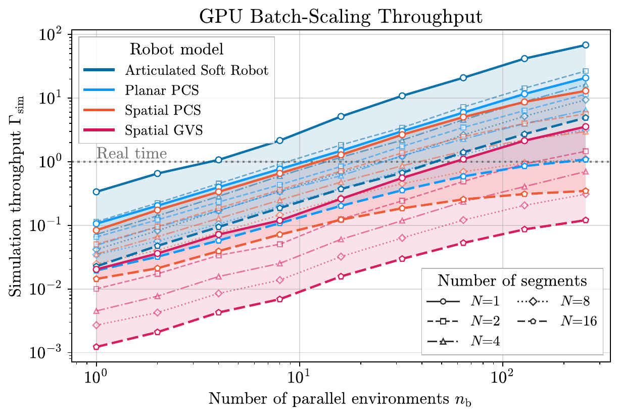
GPU batch simulation throughput for articulated, PCS, and GVS models as the leading batch size increases — On the reported RTX 5090 benchmark, scaling the leading batch size from 1 to 256 yields up to 234.6× higher simulation throughput.

The exact scaling depends on the model, number of links or segments, hardware, and discretization. Under the paper's settings, the articulated models show the strongest scaling, while the more expensive spatial PCS and GVS models still benefit substantially from batching.

Application case studies¶

1. Static-equilibrium system identification¶

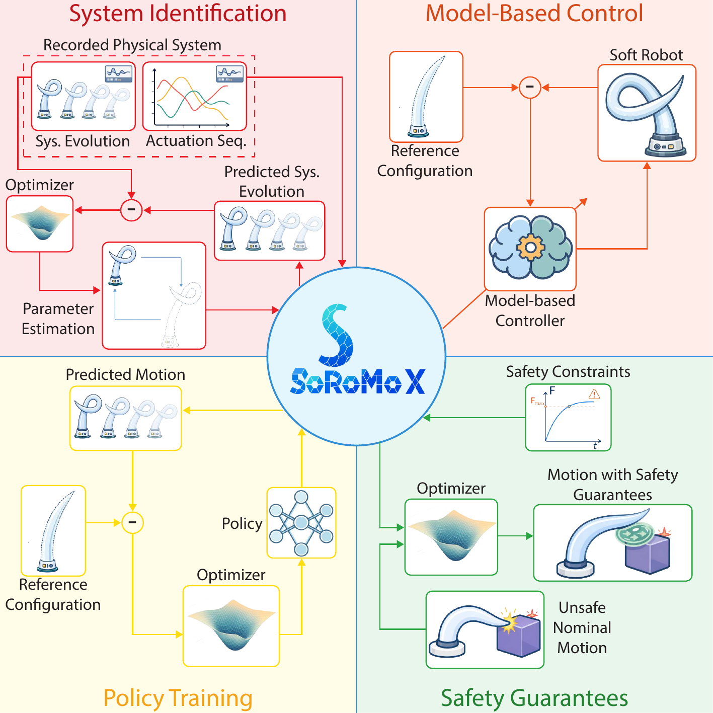
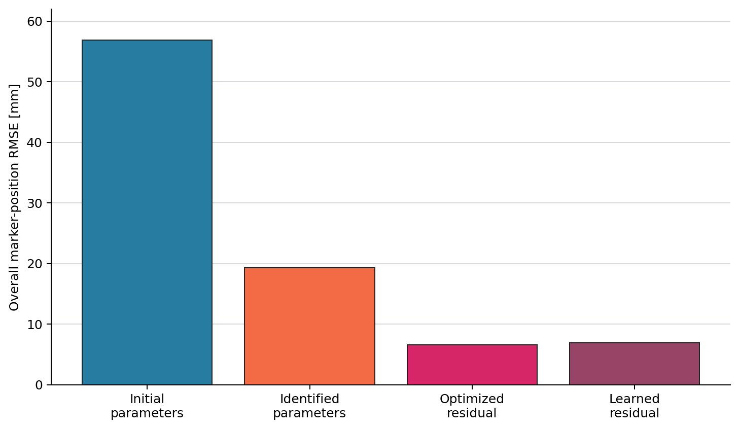
This study differentiates through a two-link GVS model to identify Young's modulus, Poisson's ratio, and mass density from static marker measurements of a conical tendon-driven arm. Optimizing the physical parameters reduces the aggregate marker-position RMSE from 56.9 mm to 19.3 mm, an improvement of about 66%.

2. Residual-force learning¶

Using the same differentiable static-equilibrium model, the study first estimates input-dependent residual generalized forces and then trains a neural network to predict them. The optimized and learned residuals reduce the overall marker RMSE to 6.6 mm and 6.9 mm, respectively.

Overall marker-position error for initial parameters, identified physical parameters, optimized residual forces, and neural-network-predicted residual forces — Shared result from the paper's static-equilibrium identification and residual-learning studies.

3. Model-based control¶

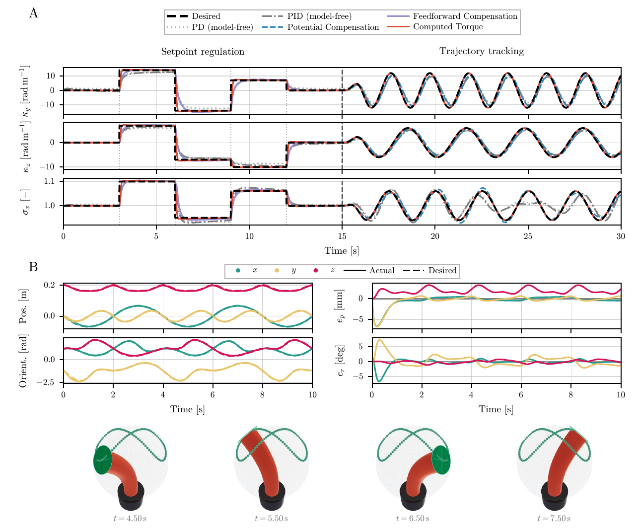
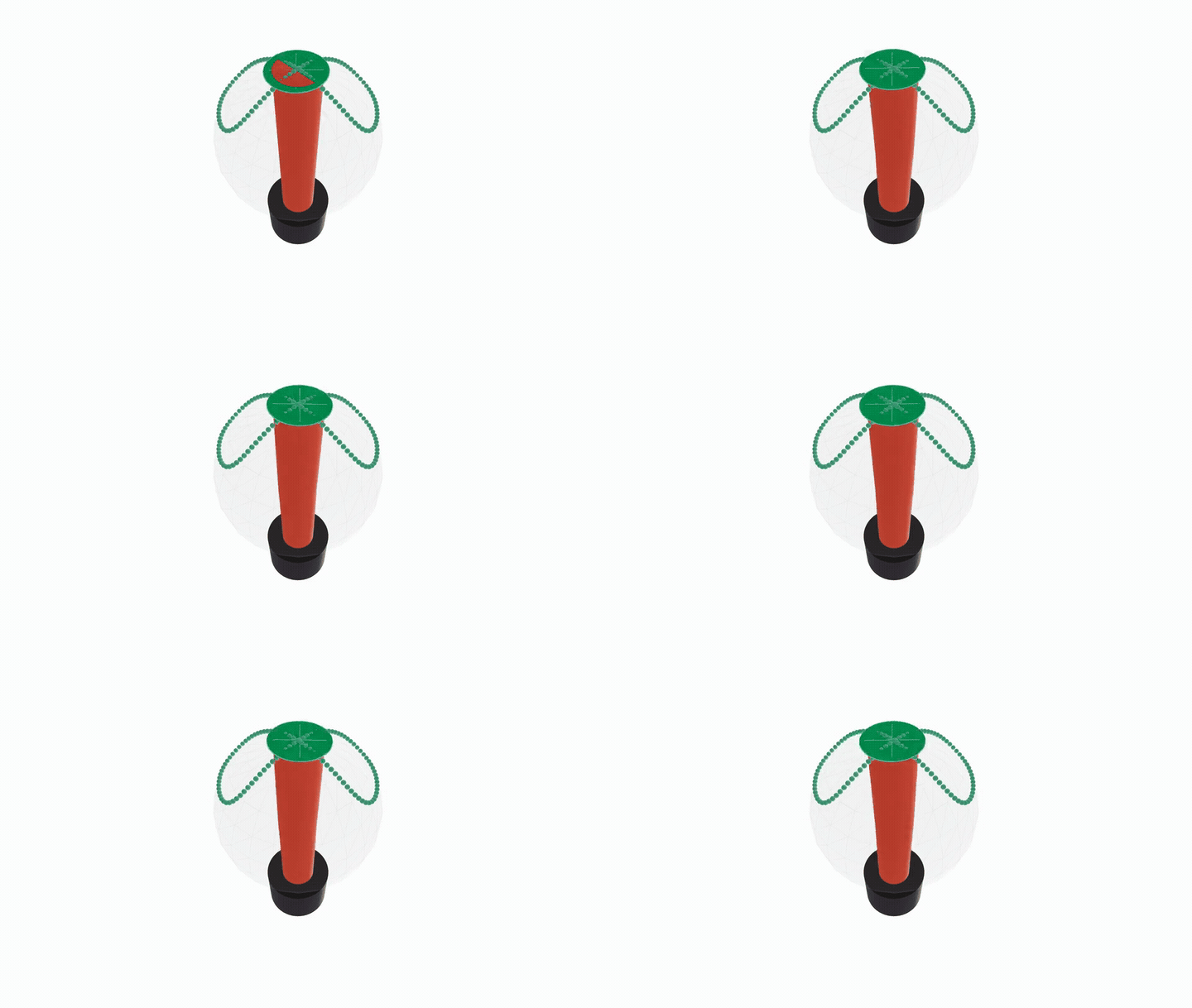
This study exercises the quantities exposed by the common model interface. A one-segment spatial PCS robot compares model-free PD/PID control with potential, feedforward, and computed-torque compensation; a fully actuated two-segment PCS robot tracks a spherical figure-eight pose trajectory with operational-space impedance control. The operational-space example reports 2.84 mm position RMSE and 2.29° orientation RMSE.

Configuration-space and operational-space model-based control results for spatial PCS robots — Paper results for configuration-space regulation/tracking and operational-space pose tracking.

4. Control-gain optimization¶

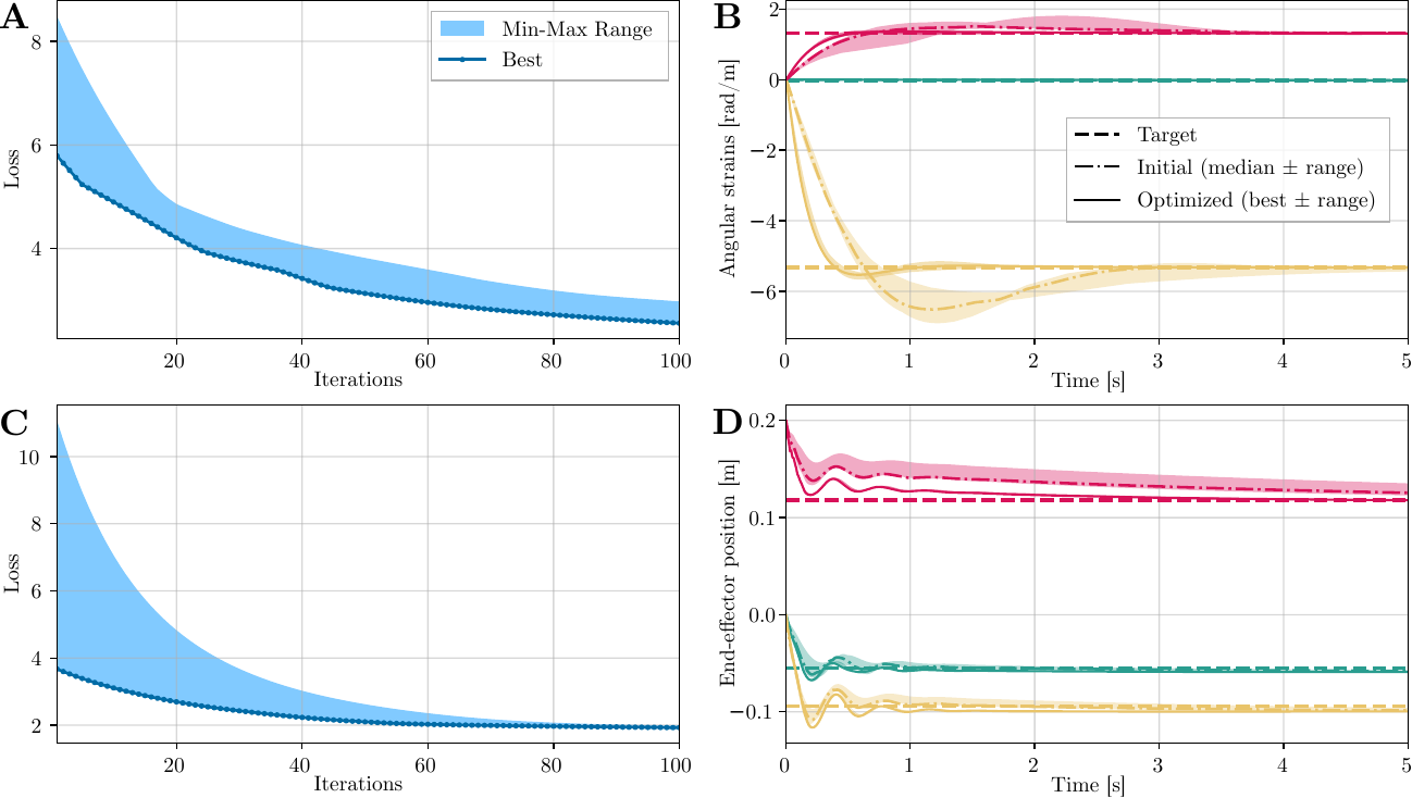
Here, gradients are propagated through full closed-loop rollouts while several gain initializations are evaluated in parallel. For actuation-space and operational-space control, the optimized losses decrease by 62% and 57%, respectively, relative to their initial median values.

Loss convergence and closed-loop responses for actuation-space and operational-space controller-gain optimization — Paper results for batched, differentiable control-gain optimization.

5. Safety-constrained control¶

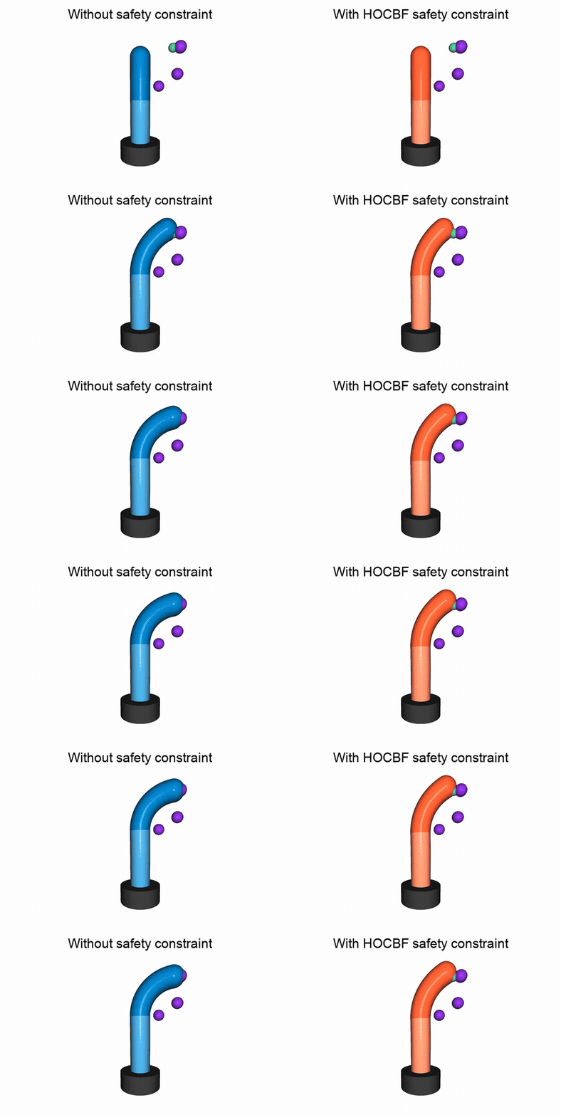
The safety study uses differentiable PCS kinematics and dynamics to formulate high-order control Lyapunov and control barrier function constraints. The safety-unaware controller reaches about 33.5 N of pairwise normal force. The HOCBF-constrained controller stays at or below the prescribed 5 N limit while accepting a larger final goal distance.

6. Parallel reinforcement learning¶

The final study vectorizes tendon-driven PCS environments on a GPU for PPO training. The trained policy reaches a 6.19 mm final mean tracking error and a 91.4% step-wise success rate. The reported 4× and 7× training speedups at 256 and 512 environments relative to the CPU PyElastica baseline jointly reflect model formulation, JIT compilation, hardware acceleration, and rollout parallelization.

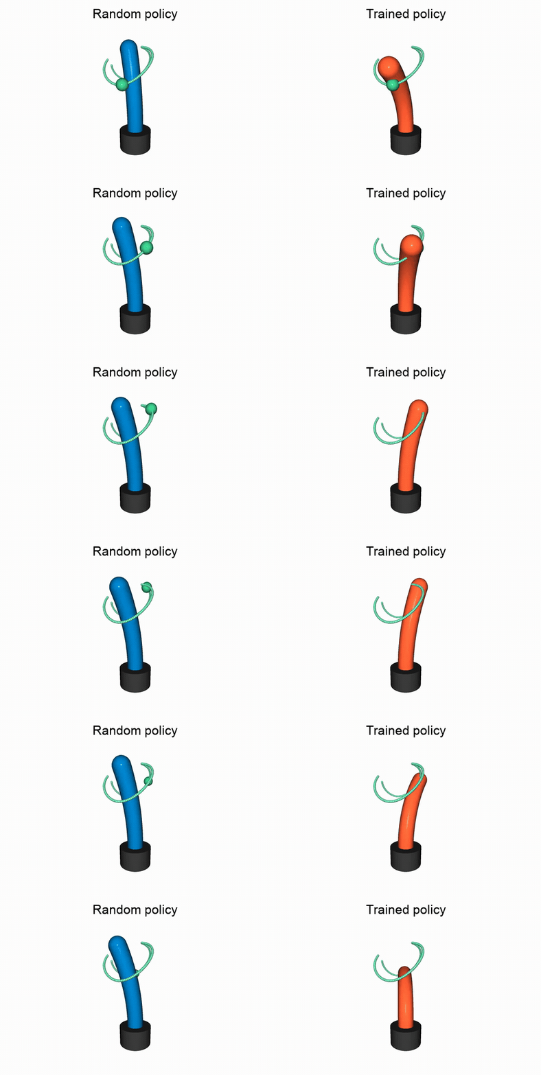
Soromox can roll out many soft-robot environments in parallel, accelerating the experience collection that dominates reinforcement-learning training. The animation below visualizes a trained policy acting simultaneously in 64 independently simulated environments.

Reproducing the results¶

The paper_results/ directory contains experiment entry points, canonical outputs, and workflow-specific notes. Install its dependencies from an editable checkout:

python -m pip install -e ".[paper_results]"

Start with the README nearest to the experiment you want to reproduce. Record the SoRoMoX version, hardware, solver configuration, and random seed with new results. For package setup, see Installation.

If you publish work based on these models or results, follow the Citation guide.